Solving the Kohn–Sham equations requires representing the single-particle orbitals $\phi_i(\mathbf{r})$ numerically. There are two complementary choices to be made:
- How to expand the orbitals — the choice of basis set.
- How to treat the core electrons — full all-electron treatment, or replace the core with a pseudopotential (PP) or projector augmented wave (PAW) potential.
These choices profoundly affect computational cost, accuracy, and the type of system tractable. This chapter develops the theory behind the most common approaches and provides practical guidance on convergence.
Basis Set Expansion
The KS orbital $\phi_i(\mathbf{r})$ is an element of an infinite-dimensional Hilbert space. In practice, it is expanded in a finite basis ${f_\mu(\mathbf{r})}$: \begin{equation} \phi_i(\mathbf{r}) = \sum_\mu c_{i\mu}\, f_\mu(\mathbf{r}), \end{equation} where the coefficients $c_{i\mu}$ are determined by diagonalising the KS Hamiltonian in this basis. The KS eigenvalue problem \eqref{eq:KS-eqn} becomes the generalised matrix eigenvalue problem: \begin{equation} \mathbf{H}_{\rm KS}\,\mathbf{c}_i = \epsilon_i\,\mathbf{S}\,\mathbf{c}_i, \end{equation} where $H_{\rm KS,\mu\nu} = \langle f_\mu | \hat{h}_{\rm KS} | f_\nu\rangle$ and $S_{\mu\nu} = \langle f_\mu | f_\nu\rangle$ is the overlap matrix. The two dominant choices are plane waves and localised (atomic-like) basis functions.
Plane-Wave Basis Sets
For crystalline solids, Bloch’s theorem dictates that KS orbitals have the form: \begin{equation} \phi_{i\mathbf{k}}(\mathbf{r}) = e^{i\mathbf{k}\cdot\mathbf{r}},u_{i\mathbf{k}}(\mathbf{r}), \end{equation} where $u_{i\mathbf{k}}(\mathbf{r})$ is lattice-periodic. The periodic part is naturally expanded in plane waves labelled by reciprocal lattice vectors $\mathbf{G}$: \begin{equation} u_{i\mathbf{k}}(\mathbf{r}) = \frac{1}{\sqrt{\Omega}}\sum_{\mathbf{G}} c_{i,\mathbf{k}+\mathbf{G}},e^{i\mathbf{G}\cdot\mathbf{r}}, \end{equation} where $\Omega$ is the unit cell volume. The basis is truncated at a kinetic energy cutoff $E_{\rm cut}$: \begin{equation} \frac{\hbar^2}{2m}|\mathbf{k}+\mathbf{G}|^2 \leq E_{\rm cut}. \end{equation}
Advantages of plane waves:
- Systematic completeness: increasing $E_{\rm cut}$ improves the basis in a controlled, unbiased way. Convergence is monitored by a single parameter.
- No basis set superposition error (BSSE): Plane waves are not centred on atoms, so the basis does not artificially lower the energy when two atoms approach.
- Efficient evaluation: The Hartree potential and charge density are related by Poisson’s equation, which is diagonal in reciprocal space. Fast Fourier transforms (FFTs) enable $\mathcal{O}(N \log N)$ switching between real and reciprocal space.
- Implemented in major codes: VASP, Quantum ESPRESSO, ABINIT, CP2K (mixed Gaussian/PW).
Disadvantages:
- All-electron calculations are impractical: Near the nuclei, KS orbitals oscillate rapidly (due to orthogonality to core states), requiring an extremely large $E_{\rm cut}$. This motivates the use of pseudopotentials or PAW (see below).
- Poor for isolated molecules: A large vacuum supercell is needed to prevent periodic images from interacting, wasting computational effort.
- Not naturally localised: Analysis (e.g. Bader charges, wannier functions) requires post-processing.
Convergence with Respect to $E_{\rm cut}$
A convergence test is mandatory in every plane-wave calculation. The procedure is:
- Fix all other parameters (cell, $k$-points, functional).
- Compute the total energy $E_{\rm tot}(E_{\rm cut})$ for a series of cutoff values.
- Identify the cutoff where $\Delta E_{\rm tot} \leq \epsilon_{\rm tol}$ (typically $1$–$5$ meV/atom).
Typical converged cutoffs: $\sim 400$–$600$ eV for GGA+PAW; $\sim 700$–$1200$ eV for norm-conserving PPs; transition metal oxides and $f$-electron systems often require higher values.
$k$-Point Sampling
In a periodic solid, the KS equations must be solved at every $\mathbf{k}$-point in the first Brillouin zone (BZ). Physical observables involve BZ integrals, e.g.:
\begin{equation} \rho(\mathbf{r}) = \frac{\Omega}{(2\pi)^3}\sum_i \int_{\rm BZ} |\phi_{i\mathbf{k}}(\mathbf{r})|^2\,d\mathbf{k}. \end{equation}In practice, the integral is replaced by a discrete sum over a finite mesh. The standard choice is the Monkhorst–Pack (MP) mesh: a uniform $N_1 \times N_2 \times N_3$ grid in reciprocal space, optionally shifted to include or exclude $\Gamma$. The total number of $k$-points is reduced by the point-group symmetry of the crystal.
Convergence with $k$-mesh density:
- Metals require denser meshes (many $k$-points near the Fermi surface): $20\times 20\times 20$ or more for simple metals.
- Semiconductors and insulators with gaps converge faster: $6\times 6\times 6$ is often sufficient.
- A smearing method (Methfessel–Paxton, Fermi–Dirac, or Gaussian) is applied to the occupation numbers for metals to accelerate convergence.
The $k$-point density and $E_{\rm cut}$ must be converged independently and jointly: the two parameters interact through the density, so a joint convergence test (varying both) is the most rigorous approach.
Localised Basis Sets
An alternative to plane waves is to expand orbitals in atom-centred functions that mimic the shape of atomic orbitals. Each basis function $f_\mu(\mathbf{r}) = f_\mu(|\mathbf{r}-\mathbf{R}_A|)$ is centred on atom $A$.
Gaussian-Type Orbitals (GTOs)
GTOs take the form $f(r) = r^l e^{-\alpha r^2} Y_l^m(\hat{\mathbf{r}})$, where $\alpha$ is the exponent and $Y_l^m$ is a real spherical harmonic. Multi-Gaussian contractions are used: \begin{equation} f_\mu(r) = \sum_k d_{\mu k},g_k(r,\alpha_k). \end{equation}
GTOs are the standard in quantum chemistry codes (Gaussian, CRYSTAL, FHI-aims). Common basis set families: 6-31G, cc-pVDZ/TZ, def2-TZVP. The acronyms encode the contraction scheme; “triple-zeta” basis sets use three groups of Gaussians per angular momentum channel and are typically converged for production calculations. Diffuse functions (denoted by $+$ or “aug-”) are important for anions and excited states.
Numerical Atomic Orbitals (NAOs)
NAOs use numerically tabulated radial functions, typically derived from atomic DFT calculations. They are compact (strictly localised beyond a cutoff radius) and efficient for large-scale calculations. Used in FHI-aims (numeric all-electron), SIESTA, OpenMX.
Advantages of localised bases:
- Efficient for molecules and non-periodic systems (no vacuum padding needed).
- Sparse Hamiltonian and overlap matrices enable $\mathcal{O}(N)$ scaling algorithms.
- Natural interface with chemical intuition (orbital populations, Mulliken/Löwdin charges).
Disadvantages:
- Basis set superposition error (BSSE): When two fragments approach, each borrows basis functions from the other, artificially lowering the energy. The counterpoise correction (Boys–Bernardi) partially remedies this.
- Incompleteness: The basis is not systematically improvable by a single parameter; basis quality depends on the choice of exponents and contraction.
- Egg-shaped convergence: Difficult to converge to the complete basis set (CBS) limit.
Core Electrons: Three Strategies
Relativistic and strongly oscillating core orbitals are expensive to represent and barely participate in chemistry or bonding. Three strategies exist for handling them.
All-Electron (AE) Calculations
All electrons, including core, are treated explicitly. Mandatory when:
- Core–valence interactions are chemically important (e.g. hyperfine coupling, NMR shifts, X-ray spectra).
- High-accuracy benchmarks are required.
- Working with very light elements (H, Li) where “core” electrons don’t exist.
Examples: FHI-aims (NAO), WIEN2k (LAPW), FLEUR.
Norm-Conserving Pseudopotentials (NCPP)
The core electrons are replaced by an effective potential $V_{\rm PP}(\mathbf{r})$ that reproduces the scattering properties of the full ionic potential in the valence region. The pseudo-wavefunction $\tilde{\phi}_l(r)$ agrees with the true all-electron wavefunction $\phi_l(r)$ outside a cutoff radius $r_c$: \begin{equation} \tilde{\phi}_l(r) = \phi_l(r), \quad r > r_c. \end{equation}
The norm-conservation condition requires: \begin{equation} \int_0^{r_c} |\tilde{\phi}_l(r)|^2 r^2,dr = \int_0^{r_c} |\phi_l(r)|^2 r^2,dr, \end{equation} ensuring that the charge inside $r_c$ is preserved and that the logarithmic derivatives (which control scattering) match at $r_c$. The Hamann–Schlüter–Chiang (HSC) and Troullier–Martins (TM) schemes are standard constructions.
NCPPs typically require $E_{\rm cut} \sim 60$–$100$ Ry and are used in codes such as Quantum ESPRESSO and ABINIT.
Ultrasoft Pseudopotentials (USPP)
The ultrasoft pseudopotential (Vanderbilt, 1990) relaxes the norm-conservation condition, allowing smoother pseudo-wavefunctions that require much lower plane-wave cutoffs ($E_{\rm cut} \sim 25$–$40$ Ry). The pseudo-wavefunction $\tilde{\phi}_l(r)$ is permitted to deviate from the all-electron $\phi_l(r)$ even for $r > r_c^{\rm soft}$, producing a softer nodeless function.
The missing charge that would violate the norm-conservation sum rule is compensated by augmentation charges $Q_{nm}(\mathbf{r})$ added to the density:
\begin{equation} \rho(\mathbf{r}) = \sum_i |\tilde{\phi}_i(\mathbf{r})|^2 + \sum_a\sum_{nm} \rho_{nm}^a\,Q_{nm}^a(\mathbf{r}), \end{equation}where $\rho_{nm}^a = \sum_i \langle\tilde{\phi}_i|\tilde{p}_n^a\rangle\langle\tilde{p}_m^a|\tilde{\phi}_i\rangle$ are the occupancy matrices for atom $a$, and $Q_{nm}^a(\mathbf{r})$ are localised functions inside the augmentation sphere that carry the missing charge. The generalised eigenvalue problem that results from USPP differs from the standard KS equation, requiring a modified orthonormality condition; however, this adds negligible overhead in practice.
USPP is available in Quantum ESPRESSO and CASTEP and offers an excellent cost-to-accuracy ratio for most elements.
Projector Augmented Wave (PAW) Method
The PAW method (Blöchl, 1994) is the most rigorous of the pseudopotential-like approaches and is now the default in most major plane-wave codes. It can be understood as a generalisation of USPP that is formally equivalent to an all-electron calculation.
The PAW Transformation
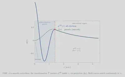
PAW introduces a linear transformation operator $\hat{\mathcal{T}}$ that maps smooth, computationally convenient pseudo-wavefunctions $|\tilde{\Psi}_i\rangle$ onto the true all-electron wavefunctions $|\Psi_i\rangle$: \begin{equation} |\Psi_i\rangle = \hat{\mathcal{T}},|\tilde{\Psi}_i\rangle. \label{eq:PAW-transform} \end{equation}
Inside the augmentation sphere of radius $r_c^a$ centred on each atom $a$, the smooth pseudo-wavefunction is a poor approximation to the oscillatory all-electron wavefunction. The transformation $\hat{\mathcal{T}}$ corrects for this, atom by atom: \begin{equation} \hat{\mathcal{T}} = \mathbf{1} + \sum_a \hat{\mathcal{T}}^a, \qquad \hat{\mathcal{T}}^a = \sum_{n} \left(|\phi_n^a\rangle - |\tilde{\phi}_n^a\rangle\right)\langle\tilde{p}_n^a|, \label{eq:PAW-T} \end{equation} where:
- $|\phi_n^a\rangle$ are all-electron partial waves — solutions of the radial Schrödinger equation for the isolated atom $a$ at reference energies, labelled by $n = (l, m, \epsilon_{\rm ref})$.
- $|\tilde{\phi}_n^a\rangle$ are smooth pseudo partial waves that match $|\phi_n^a\rangle$ outside $r_c^a$ but are nodeless and smooth inside.
- $\langle\tilde{p}_n^a|$ are projector functions localised inside $r_c^a$, dual to the pseudo partial waves: $\langle\tilde{p}_n^a|\tilde{\phi}m^a\rangle = \delta{nm}$.
The transformation acts as follows: when $\hat{\mathcal{T}}$ is applied to $|\tilde{\Psi}_i\rangle$, the projectors $\langle\tilde{p}_n^a|$ measure the overlap of the smooth wavefunction with the partial waves in each augmentation sphere, and the difference $(|\phi_n^a\rangle - |\tilde{\phi}_n^a\rangle)$ restores the all-electron character inside that sphere. Outside all augmentation spheres, $\hat{\mathcal{T}}^a = 0$ and the smooth wavefunction is used directly.
Reconstruction of the All-Electron Density
The all-electron charge density is: \begin{equation} \rho(\mathbf{r}) = \tilde{\rho}(\mathbf{r}) + \rho^1(\mathbf{r}) - \tilde{\rho}^1(\mathbf{r}), \label{eq:PAW-density} \end{equation} where each term has a specific role:
$\tilde{\rho}(\mathbf{r}) = \sum_i f_i,|\tilde{\Psi}_i(\mathbf{r})|^2$ is the smooth pseudo-density, computed from the plane-wave-expanded pseudo-wavefunctions throughout the entire cell. This is the computationally cheap term, evaluated with FFTs.
$\rho^1(\mathbf{r}) = \sum_a\sum_{nm}\rho_{nm}^a,\phi_n^a(\mathbf{r})\phi_m^a(\mathbf{r})$ is the on-site all-electron density, reconstructed analytically from the all-electron partial waves inside the augmentation spheres. Here $\rho_{nm}^a = \sum_i f_i\langle\tilde{\Psi}_i|\tilde{p}_n^a\rangle\langle\tilde{p}_m^a|\tilde{\Psi}_i\rangle$ are the occupation matrices that quantify the partial-wave character of each KS orbital at each atom.
$\tilde{\rho}^1(\mathbf{r}) = \sum_a\sum_{nm}\rho_{nm}^a,\tilde{\phi}_n^a(\mathbf{r})\tilde{\phi}_m^a(\mathbf{r})$ is the on-site pseudo-density, which subtracts the smooth-wavefunction contribution inside the augmentation spheres so it is not double-counted with $\tilde{\rho}$.
The total energy is decomposed in the same three-part way. The smooth part is evaluated in reciprocal space via FFTs; the on-site parts are computed analytically on radial grids inside each augmentation sphere. This decomposition is the key to PAW’s efficiency: the expensive oscillatory core region is handled on a small radial grid, while the smooth interstitial region uses the standard plane-wave machinery.
The PAW Total Energy
The total energy functional in PAW is: \begin{equation} E = \tilde{E} + E^1 - \tilde{E}^1, \end{equation}
where $\tilde{E}$ is the energy of the pseudo-system (computed with plane waves), $E^1$ is the all-electron on-site energy inside the augmentation spheres, and $\tilde{E}^1$ is the corresponding pseudo on-site energy that prevents double-counting. The KS equations derived from this functional take the form of a generalised eigenvalue problem: \begin{equation} \hat{\tilde{H}}\,|\tilde{\Psi}_i\rangle = \epsilon_i\,\hat{S}\,|\tilde{\Psi}_i\rangle, \end{equation}
where $\hat{\tilde{H}}$ is the smooth KS Hamiltonian (including on-site corrections) and $\hat{S} = \mathbf{1} + \sum_a\sum_{nm}({\langle\tilde{p}_n^a|\tilde{p}_m^a\rangle_{\rm AE} - \delta_{nm}})|\tilde{p}_m^a\rangle\langle\tilde{p}_n^a|$ is the overlap operator that enforces the correct normalisation of the all-electron wavefunctions.
Strengths of PAW
- Formally all-electron: The full all-electron density is available in the augmentation spheres through equation \eqref{eq:PAW-density}. This gives direct access to hyperfine parameters, electric field gradients, NMR chemical shifts, and core-level binding energies.
- Low $E_{\rm cut}$: The smooth part $|\tilde{\Psi}i\rangle$ requires $E{\rm cut} \sim 400$–$600$ eV (VASP), similar to USPP, far below what a true all-electron plane-wave calculation would need.
- Transferability: The partial waves are atom-specific but not system-specific; the same PAW dataset works well across different chemical environments, unlike empirically fitted NCPP.
- Extensibility: The occupation matrices $\rho_{nm}^a$ are a natural handle for DFT+U and hybrid functional implementations.
Limitations of PAW
- Fixed augmentation spheres: If $r_c^a$ is too small, the smooth part is not genuinely smooth; if too large, augmentation spheres on adjacent atoms overlap, invalidating the non-overlapping sphere assumption. Standard VASP PAW datasets are designed to avoid overlap for typical bond lengths, but this must be verified under compression.
- Linearisation of the partial wave expansion: PAW is exact only if the partial wave basis ${|\phi_n^a\rangle}$ is complete within the augmentation sphere. For highly ionic environments or unusual oxidation states, a larger partial wave set or scattering energies closer to the occupied states may be needed. VASP provides both standard and “hard” PAW datasets for such cases.
Comparison of core-electron strategies:
| Method | $E_{\rm cut}$ (typical) | Core accuracy | Access to core density | Cost | Default in |
|---|---|---|---|---|---|
| NCPP | $60$–$100$ Ry | Good (outside $r_c$) | No | Moderate | QE, ABINIT |
| USPP | $25$–$40$ Ry | Good (valence) | No | Low | QE, CASTEP |
| PAW | $30$–$50$ Ry | Excellent (AE in spheres) | Yes | Low–moderate | VASP, QE |
| All-electron | $\gg 100$ Ry | Exact | Yes | High | FHI-aims, WIEN2k |
Practical Convergence Protocol
A rigorous DFT calculation requires the following checks, performed in order:
$E_{\rm cut}$ convergence: Increase the plane-wave cutoff until the total energy changes by less than $1$–$2$ meV/atom. Use the converged cutoff for all subsequent calculations.
$k$-mesh convergence: Increase the Monkhorst–Pack grid density until the total energy and the quantity of interest (e.g. magnetic moment, band gap) are converged. Report the converged grid as $N_1 \times N_2 \times N_3$.
Supercell size (for defects, surfaces, molecules): Increase the cell size until the interaction between periodic images is negligible ($\Delta E < 1$ meV/defect).
SCF convergence criterion: Tighten the SCF energy tolerance to $\sim 10^{-6}$ eV for energy differences; $\sim 10^{-7}$ eV for forces or stress calculations.
Structural convergence: Relax ionic positions until forces are below $0.01$–$0.02$ eV/Å; relax the cell until stresses are below $0.1$ kbar.
Failure to converge any one of these can produce errors that dwarf those from the choice of XC functional. Convergence tests must be performed for each new system class; results from one system cannot be assumed transferable.
Outlook
With the KS equations specified, the XC functional chosen, and the basis and pseudopotential converged, we have all the ingredients for a standard spin-unpolarised DFT calculation. The next chapter extends the framework to spin-polarised systems, which are essential for magnetic materials and the study of exchange coupling in Heusler alloys and related compounds.