In the Kohn–Sham framework, all the complexity of many-body quantum mechanics is concentrated in a single term: the exchange-correlation energy $E_{\rm xc}[\rho]$. If the exact $E_{\rm xc}$ were known, DFT would be formally exact. In practice it must be approximated, and six decades of development have produced a rich hierarchy of approximations.
Rather than presenting this hierarchy as a list of progressively better recipes, this chapter derives it from two systematic expansions, each anchored at a different exactly-known limit:
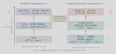
A spatial gradient expansion around the uniform electron gas (UEG) — the only interacting electron system for which $E_{\rm xc}$ is known exactly. Expanding in powers of the dimensionless density gradient generates the semi-local hierarchy: LDA → GGA → meta-GGA.
A coupling-constant expansion around the non-interacting KS limit — the point at which the exact exchange is known analytically. Expanding in powers of the interaction strength generates the non-local hierarchy: GGA → hybrid → double-hybrid.
These two series are orthogonal: the first improves the local description of the XC hole shape; the second improves its non-local content. Understanding their structure turns the choice of functional from a matter of recipe-following into a matter of physics.
Formal Definition and the Two Reference Points
The XC Hole
The XC energy is defined by the decomposition introduced in Chapter 3: \begin{equation} E_{\rm xc}[\rho] = (T[\rho] - T_s[\rho]) + (V_{ee}[\rho] - E_{\rm H}[\rho]). \label{eq:Exc-def} \end{equation}
An equivalent and physically transparent form expresses $E_{\rm xc}$ in terms of the exchange-correlation hole $n_{\rm xc}(\mathbf{r}, \mathbf{r}’)$ — the depletion of electron density at $\mathbf{r}’$ caused by the presence of an electron at $\mathbf{r}$: \begin{equation} E_{\rm xc}[\rho] = \frac{1}{2}\iint \frac{\rho(\mathbf{r}),n_{\rm xc}(\mathbf{r},\mathbf{r}’)}{|\mathbf{r}-\mathbf{r}’|},d\mathbf{r},d\mathbf{r}’. \end{equation}
The exact XC hole satisfies two rigorous constraints: \begin{equation} n_{\rm xc}(\mathbf{r},\mathbf{r}’) \leq 0, \qquad \int n_{\rm xc}(\mathbf{r},\mathbf{r}’),d\mathbf{r}’ = -1. \label{eq:hole-sumrule} \end{equation}
The second relation — the sum rule — encodes the fact that each electron excludes exactly one unit of charge from its neighbourhood. Approximations that satisfy this constraint tend to benefit from systematic error cancellation even when the detailed shape of the hole is wrong, which explains the surprising accuracy of LDA despite its crude derivation.
The Two Exactly-Known Limits
Two limits of $E_{\rm xc}$ are known exactly and serve as expansion points.
Limit 1 — Uniform electron gas ($s = 0$): When the density is spatially uniform, $\rho(\mathbf{r}) = \bar\rho$, the XC energy per electron $\varepsilon_{\rm xc}(\bar\rho)$ is known with essentially arbitrary precision from quantum Monte Carlo simulations (Ceperley–Alder, 1980). The exchange component is analytic (Dirac, 1930). This is the natural anchor for a Taylor series in density variations.
Limit 2 — Non-interacting KS limit ($\lambda = 0$): Via the adiabatic connection, the XC energy is written as an integral over a coupling constant $\lambda \in [0,1]$ that smoothly scales the electron–electron interaction from zero (the KS system) to its physical value: \begin{equation} E_{\rm xc}[\rho] = \int_0^1 W_{\rm xc}^\lambda[\rho]\,d\lambda, \qquad W_{\rm xc}^\lambda = \langle\Psi^\lambda|\hat{V}_{ee}|\Psi^\lambda\rangle - E_{\rm H}[\rho], \label{eq:adiabatic} \end{equation}
where $\Psi^\lambda$ is the ground state with the same density $\rho$ but interaction scaled by $\lambda$. At $\lambda = 0$, $\Psi^0$ is the KS Slater determinant and $W_{\rm xc}^0 = E_{\rm x}^{\rm exact}$ is known analytically. This is the natural anchor for a Taylor series in interaction strength.
The First Taylor Series: Gradient Expansion and Semi-Local Functionals
The Dimensionless Gradient and the GEA
For a slowly varying density, we measure spatial variation by the reduced density gradient: \begin{equation} s(\mathbf{r}) = \frac{|\nabla\rho(\mathbf{r})|}{2k_F(\mathbf{r}),\rho(\mathbf{r})}, \qquad k_F(\mathbf{r}) = (3\pi^2\rho(\mathbf{r}))^{1/3}, \label{eq:s-def} \end{equation} where $k_F$ is the local Fermi wavevector. The parameter $s$ measures the density gradient in units of the local electron wavelength: $s = 0$ for the UEG; $s \sim 0.5$–$3$ in typical valence regions; $s \to \infty$ in exponentially decaying density tails.
The formal gradient expansion approximation (GEA) from many-body perturbation theory gives the systematic Taylor series in $s^2$ (odd powers vanish by symmetry): \begin{equation} E_{\rm xc}^{\rm GEA}[\rho] = \int \rho,\varepsilon_{\rm xc}^{\rm UEG}(\rho),d\mathbf{r} + \int C_{\rm xc}(\rho),s^2,\rho,d\mathbf{r} + \mathcal{O}(s^4), \label{eq:GEA} \end{equation} where $C_{\rm xc}(\rho)$ is a density-dependent coefficient computable from perturbation theory.
Rung 0: LDA — Zeroth Order
Truncating \eqref{eq:GEA} at zeroth order ($s^0$) gives the local density approximation: \begin{equation} \boxed{E_{\rm xc}^{\rm LDA}[\rho] = \int \varepsilon_{\rm xc}^{\rm UEG}(\rho(\mathbf{r})),\rho(\mathbf{r}),d\mathbf{r}.} \label{eq:LDA} \end{equation}
The exchange part is analytic (Dirac, 1930): \begin{equation} \varepsilon_{\rm x}^{\rm UEG}(\rho) = -\frac{3}{4}!\left(\frac{3}{\pi}\right)^{!1/3}!\rho^{1/3}. \end{equation} The correlation $\varepsilon_{\rm c}(\rho)$ is parameterised from QMC data: the Perdew–Wang (PW92) and Vosko–Wilk–Nusair (VWN) parameterisations are most common.
Why LDA works better than a zeroth-order truncation deserves. The LDA XC hole is that of the UEG, which satisfies the sum rule \eqref{eq:hole-sumrule} by construction. Even when the detailed angular shape of the hole is wrong, the spherically averaged hole — which is what determines $E_{\rm xc}$ via a radial integral — is described well. This is systematic error cancellation rooted in constraint satisfaction, not coincidence.
Known systematic errors: overbinds (cohesive energies $+1$–$2$ eV/atom); underestimates lattice constants ($-1$–$3%$); underestimates band gaps ($-40%$); no dispersion.
When to use LDA: Phonons and structural properties of simple and alkali metals, where the electron gas is nearly uniform and the error cancellation is most favourable.
Why the Raw GEA Fails
The $\mathcal{O}(s^2)$ term in \eqref{eq:GEA} does not improve on LDA — it makes things worse. The GEA correction introduces oscillations in the XC hole at large $|\mathbf{r}-\mathbf{r}’|$ (where $s$ is large), causing the hole to become positive and violating $n_{\rm xc} \leq 0$ and the $-1$ sum rule in the density tails. This is a classical example of a Taylor series that diverges when the expansion parameter is not uniformly small: $s \to \infty$ in the tail of any finite system.
Rung 1: GGA — Constrained Resummation of the Gradient Series
Rather than truncating \eqref{eq:GEA}, the generalised gradient approximation writes the XC energy in the enhancement factor form: \begin{equation} \boxed{E_{\rm xc}^{\rm GGA}[\rho] = \int \varepsilon_{\rm xc}^{\rm UEG}(\rho),F_{\rm xc}(\rho, s),\rho,d\mathbf{r},} \label{eq:GGA} \end{equation} where $F_{\rm xc}(\rho, s)$ is a dimensionless enhancement factor. GGA is not the $\mathcal{O}(s^2)$ truncation — it is a constrained resummation that reproduces the correct $s^2$ behaviour near $s = 0$ while satisfying exact constraints for all $s$.
PBE (Perdew–Burke–Ernzerhof, 1996) determines $F_{\rm xc}$ by imposing:
- $F_{\rm xc} \to 1$ as $s \to 0$: recovers LDA, consistent with the UEG limit.
- $\partial F_{\rm xc}/\partial(s^2)|_0 = \mu$: matches the GEA gradient coefficient, ensuring consistency with perturbation theory at small $s$.
- Cutoff at large $s$: $F_{\rm xc}$ saturates rather than growing without bound, enforcing the sum rule $\int n_{\rm x}^{\rm GGA},d\mathbf{r}’ = -1$ even in the density tails. This is precisely the correction to the GEA failure above.
- Lieb–Oxford bound: $E_{\rm xc}^{\rm GGA} \geq -1.679\int\rho^{4/3},d\mathbf{r}$, a rigorous lower bound satisfied for all $s$.
The explicit PBE exchange enhancement factor is: \begin{equation} F_{\rm x}^{\rm PBE}(s) = 1 + \kappa - \frac{\kappa}{1 + \mu s^2/\kappa}, \qquad \kappa = 0.804,\quad \mu = 0.2195, \end{equation} where both parameters are fixed by constraints, not by fitting to data. PBE has zero empirical parameters.
LDA vs. PBE:
| Property | LDA | PBE |
|---|---|---|
| Lattice constants | $-1$ to $-3%$ | $+1$ to $+2%$ |
| Atomisation energies | $+30$ kcal/mol | $+10$ kcal/mol |
| Band gaps | $-40%$ | $-40%$ |
| Hydrogen bonds | Reasonable | Good |
| Van der Waals | Very poor | Poor |
The band gap error is essentially unchanged between LDA and PBE: it originates not in the gradient expansion but in the missing derivative discontinuity of the exact XC potential at integer electron number, which no semi-local functional can capture.
PBEsol restores the exact second-order GEA gradient coefficient for exchange (replacing $\mu$ with the perturbation-theory value), improving lattice constants for dense solids at the cost of atomisation energy accuracy. It is preferred for crystallographic properties.
Rung 2: Meta-GGA — Encoding $\mathcal{O}(s^4)$ Through $\tau$
The gradient expansion \eqref{eq:GEA} can in principle be extended to $\mathcal{O}(s^4)$, which involves second spatial derivatives $\nabla^2\rho$. However, $\nabla^2\rho$ included directly reintroduces oscillatory behaviour in the density tails. The kinetic energy density: \begin{equation} \tau(\mathbf{r}) = \frac{1}{2}\sum_i f_i,|\nabla\phi_i(\mathbf{r})|^2 \end{equation} encodes the same fourth-order gradient information without the oscillation pathology, since it involves the square of orbital gradients rather than their Laplacian. The two quantities are related by: \begin{equation} \tau = \tau^W + \tau^{\rm UEG} + \mathcal{O}(\nabla^4\rho), \qquad \tau^W = \frac{|\nabla\rho|^2}{8\rho},\quad \tau^{\rm UEG} = \frac{3}{10}(3\pi^2)^{2/3}\rho^{5/3}. \end{equation}
The meta-GGA adds $\tau$ as a third ingredient: \begin{equation} \boxed{E_{\rm xc}^{\rm mGGA}[\rho] = \int \varepsilon_{\rm xc}(\rho,,s,,\alpha),\rho,d\mathbf{r},} \end{equation} organised around the iso-orbital indicator: \begin{equation} \alpha(\mathbf{r}) = \frac{\tau(\mathbf{r}) - \tau^W(\mathbf{r})}{\tau^{\rm UEG}(\mathbf{r})}, \label{eq:alpha} \end{equation} whose physical content follows directly from its definition:
- $\alpha = 0$: $\tau = \tau^W$, which holds exactly for a single orbital. Signals a covalent bond, a core region, or any single-orbital-dominated region. The functional should be exact for one electron.
- $\alpha = 1$: $\tau = \tau^W + \tau^{\rm UEG}$, which holds for the UEG. The functional should recover LDA.
- $\alpha \gg 1$: many KS orbitals contribute to $\tau$ but the density varies slowly. Signals weak overlap between closed-shell fragments — the van der Waals regime.
SCAN (Strongly Constrained and Appropriately Normed; Sun, Ruzsinszky, Perdew, 2015) constructs $\varepsilon_{\rm xc}(\rho, s, \alpha)$ to satisfy simultaneously all 17 exact constraints applicable to a semi-local functional — the first functional to achieve this. r²SCAN (Furness et al., 2020) is a numerically regularised variant that avoids a discontinuity in $\partial\varepsilon_{\rm xc}/\partial\alpha$ at $\alpha = 0$ that causes SCF convergence difficulties in plane-wave codes; it is the recommended choice for practical calculations.
Key improvements over PBE: lattice constants improved to $\sim 0.3%$; atomisation energies improved by $\sim 30%$; qualitatively correct van der Waals interactions for layered materials from the $\alpha \gg 1$ switching (though quantitatively insufficient without dispersion corrections); better magnetic exchange couplings and transition metal oxide band gaps.
The Second Taylor Series: Coupling-Constant Expansion and Non-Local Functionals
The semi-local functionals above improve the spatial description of the XC hole but remain fundamentally local: $\varepsilon_{\rm xc}$ at $\mathbf{r}$ depends only on quantities at $\mathbf{r}$. A qualitatively different class of improvement comes from the second Taylor series.
Expanding $W_{\rm xc}^\lambda$ Around $\lambda = 0$
We expand the adiabatic connection integrand \eqref{eq:adiabatic} in $\lambda$: \begin{equation} W_{\rm xc}^\lambda = W_{\rm xc}^0 + \lambda\left.\frac{dW_{\rm xc}^\lambda}{d\lambda}\right|{\lambda=0} + \frac{\lambda^2}{2}\left.\frac{d^2W{\rm xc}^\lambda}{d\lambda^2}\right|_{\lambda=0} + \cdots \label{eq:AC-Taylor} \end{equation}
The zeroth-order term is exactly known: \begin{equation} W_{\rm xc}^0 = E_{\rm x}^{\rm exact}[{\phi_i}] = -\frac{1}{2}\sum_{i,j}\iint\frac{\phi_i^(\mathbf{r})\phi_j(\mathbf{r})\phi_j^(\mathbf{r}’)\phi_i(\mathbf{r}’)}{|\mathbf{r}-\mathbf{r}’|},d\mathbf{r},d\mathbf{r}’. \end{equation}
The first derivative is identified by Görling–Levy (GL) perturbation theory as twice the second-order GL correlation energy $E_{\rm c}^{\rm GL2}$: \begin{equation} \left.\frac{dW_{\rm xc}^\lambda}{d\lambda}\right|{\lambda=0} = 2E{\rm c}^{\rm GL2} = -2\sum_{\substack{i < j \ a < b}} \frac{|\langle\phi_i\phi_j|\phi_a\phi_b\rangle|^2}{\epsilon_a + \epsilon_b - \epsilon_i - \epsilon_j}, \label{eq:GL2} \end{equation} where $i,j$ label occupied and $a,b$ unoccupied KS orbitals. This has the same algebraic structure as MP2 correlation but is evaluated on KS orbitals. Integrating \eqref{eq:AC-Taylor}: \begin{equation} E_{\rm xc} = E_{\rm x}^{\rm exact} + E_{\rm c}^{\rm GL2} + \frac{1}{6}\left.\frac{d^2W_{\rm xc}^\lambda}{d\lambda^2}\right|_{\lambda=0} + \cdots \label{eq:AC-integrated} \end{equation}
Each successive term is more expensive and more accurate.
Rung 3: Global Hybrid Functionals — Zeroth-Order Plus Remainder
Retaining only the zeroth-order term $E_{\rm x}^{\rm exact}$ and approximating the remainder of the $\lambda$ integral by a GGA gives the global hybrid: \begin{equation} \boxed{E_{\rm xc}^{\rm hybrid} = a,E_{\rm x}^{\rm exact} + (1-a),E_{\rm x}^{\rm GGA} + E_{\rm c}^{\rm GGA}.} \label{eq:hybrid} \end{equation}
The fraction $a$ is not a free parameter: fourth-order GL perturbation theory (Perdew, Ernzerhof, Burke, 1996) shows that for systems near the weakly correlated limit, the integrand $W_{\rm xc}^\lambda$ is nearly linear in $\lambda$, and the trapezoidal rule $(W_0 + W_1)/2$ gives $a = 1/2$. Since GGA already captures part of the $\lambda = 1$ end, the effective exact exchange weight is smaller, and GL4 gives $a = 1/4$ as the optimal parameter-free estimate.
PBE0
PBE0 implements \eqref{eq:hybrid} with $a = 1/4$ from GL4 perturbation theory and PBE as the semi-local component: \begin{equation} E_{\rm xc}^{\rm PBE0} = \frac{1}{4}E_{\rm x}^{\rm exact} + \frac{3}{4}E_{\rm x}^{\rm PBE} + E_{\rm c}^{\rm PBE}. \end{equation}
PBE0 has no empirical parameters. In the limit $a \to 0$ it recovers PBE exactly. Band gaps improve from $-40%$ (PBE) to $\sim -20%$ (PBE0), and reaction barriers improve substantially. The cost in a periodic code scales as $\mathcal{O}(N^3)$ with density fitting, making it expensive for large unit cells.
B3LYP
B3LYP (Becke, 1993) occupies the same position in the coupling-constant series but determines its three parameters $(a_0, a_x, a_c)$ empirically by fitting to the G2 molecular thermochemistry database rather than from perturbation theory: \begin{equation} E_{\rm xc}^{\rm B3LYP} = (1-a_0)E_{\rm x}^{\rm LSDA} + a_0,E_{\rm x}^{\rm exact} + a_x\Delta E_{\rm x}^{\rm B88} + (1-a_c)E_{\rm c}^{\rm VWN} + a_c,E_{\rm c}^{\rm LYP}, \end{equation} with $a_0 = 0.20$, $a_x = 0.72$, $a_c = 0.81$. The LYP correlation (Lee–Yang–Parr) is derived from the Colle–Salvetti helium atom expression, not from the UEG, so it does not reduce to $\varepsilon_{\rm c}^{\rm UEG}$ in the uniform limit. This makes B3LYP physically inconsistent for metallic systems but very well-suited to organic molecules (its fitting set): thermochemical accuracy $\sim 3$ kcal/mol, bond lengths $\sim 0.01$ Å. It should not be used for periodic metals or large-gap insulators.
The contrast between PBE0 and B3LYP is instructive: both sit at the same rung of the coupling-constant ladder, but PBE0 is constraint-derived and transferable while B3LYP is empirically optimal within its training domain.
The Spatial Structure of the Exchange Hole: Motivating Range Separation
Global hybrids apply the same fraction $a$ of exact exchange uniformly at all length scales. But the exchange hole $n_{\rm x}(\mathbf{r},\mathbf{r}’)$ behaves fundamentally differently at short and long range.
At short range ($|\mathbf{r}-\mathbf{r}’| \to 0$): the hole is deep, localised, and cusp-like. Semi-local functionals describe this region reasonably well.
At long range ($|\mathbf{r}-\mathbf{r}’| \to \infty$): the exact exchange hole of a finite system must decay as $-1/r$ to satisfy the $-1$ sum rule. This $-1/r$ tail implies that the exchange potential $V_{\rm x}(\mathbf{r}) \to -1/r$ asymptotically — a non-local behaviour that only exact exchange can reproduce; semi-local functionals decay exponentially instead.
For solids, the situation is reversed at long range: the dielectric response of the crystal screens the exchange hole so that the effective long-range decay is faster than $-1/r$. In a perfect metal, the exchange interaction is fully screened beyond the Thomas–Fermi length ($\sim 0.5$ Å), so exact long-range exchange is not only unnecessary but harmful — it produces a logarithmic divergence of the exchange potential at the Fermi surface.
This physics suggests splitting the Coulomb operator into short-range (SR) and long-range (LR) parts using the error function: \begin{equation} \frac{1}{r_{12}} = \underbrace{\frac{\mathrm{erfc}(\omega r_{12})}{r_{12}}}{\mathrm{SR}: ;\to 0\text{ as }r{12}\to\infty} + \underbrace{\frac{\mathrm{erf}(\omega r_{12})}{r_{12}}}{\mathrm{LR}: ;\to 1/r{12}\text{ as }r_{12}\to\infty}, \label{eq:range-split} \end{equation} where $\omega$ controls the crossover: $r_c \approx 1/\omega$. Different exact exchange fractions $a_{\rm SR}$ and $a_{\rm LR}$ are then applied to each part.
HSE06 — Short-Range Exact Exchange for Solids
HSE06 (Heyd–Scuseria–Ernzerhof, 2003/2006) applies exact exchange at short range only: \begin{equation} E_{\rm xc}^{\rm HSE06} = \frac{1}{4}E_{\rm x}^{\rm exact,SR}(\omega) + \frac{3}{4}E_{\rm x}^{\rm PBE,SR}(\omega) + E_{\rm x}^{\rm PBE,LR}(\omega) + E_{\rm c}^{\rm PBE}, \end{equation} with $\omega = 0.11$ bohr$^{-1}$ ($\approx 0.21$ Å$^{-1}$, crossover $\sim 5$–$10$ Å).
The limits confirm the physical motivation: $\omega \to 0$ recovers PBE0 (no screening, appropriate for molecules); $\omega \to \infty$ recovers PBE (full screening, appropriate for metals). At $\omega = 0.11$ bohr$^{-1}$, HSE06 describes the screened exchange of a typical semiconductor. Computational advantages are significant: the short-range Fock operator decays exponentially in real space, enabling $\mathcal{O}(N)$ scaling, making HSE06 tractable for unit cells of hundreds of atoms.
Performance: band gaps within $\sim 10$–$15%$ of experiment for most semiconductors; correct metallic behaviour where PBE0 fails; standard functional for band gap calculations in periodic solids.
LC-$\omega$PBE and $\omega$B97X-V — Long-Range Exact Exchange for Molecules
For isolated molecules, the physical argument is opposite: the density tails are unscreened, and the correct $-1/r$ asymptote of $V_{\rm x}$ is essential for Rydberg states and charge-transfer excitations. Long-range corrected (LC) functionals apply exact exchange at long range: \begin{equation} E_{\rm xc}^{\rm LC} = E_{\rm x}^{\rm GGA,SR}(\omega) + E_{\rm x}^{\rm exact,LR}(\omega) + E_{\rm c}^{\rm GGA}. \end{equation}
$\omega$B97X-V (Mardirossian–Head-Gordon, 2014; $a_{\rm SR} = 0.167$, $a_{\rm LR} = 1.0$, $\omega = 0.30$ Å$^{-1}$) further combines long-range correction with the non-local VV10 dispersion functional, treating van der Waals at the functional level. It ranks among the best single functionals for molecular benchmarks.
CAM-B3LYP (Yanai et al., 2004) interpolates smoothly between $a_{\rm SR} = 0.19$ and $a_{\rm LR} = 0.65$ using $\omega = 0.33$ Å$^{-1}$, retaining B3LYP’s ground-state accuracy while improving excited states.
Summary: Global and Range-Separated Hybrids
| Functional | $a_{\rm SR}$ | $a_{\rm LR}$ | $\omega$ (Å$^{-1}$) | Primary use |
|---|---|---|---|---|
| PBE0 | 0.25 | 0.25 | — | Molecules and solids (no screening) |
| B3LYP | 0.20 | 0.20 | — | Organic molecules |
| HSE06 | 0.25 | 0.00 | 0.21 | Periodic solids, large cells |
| LC-$\omega$PBE | 0.00 | 1.00 | 0.40 | Charge transfer, Rydberg |
| CAM-B3LYP | 0.19 | 0.65 | 0.33 | Molecular excited states |
| $\omega$B97X-V | 0.167 | 1.00 | 0.30 | Molecular thermochemistry + vdW |
Rung 4: Double-Hybrid Functionals — First-Order Term
Retaining both the zeroth- and first-order terms of \eqref{eq:AC-integrated} and approximating the GGA remainder for the higher orders gives the double-hybrid: \begin{equation} \boxed{E_{\rm xc}^{\rm DH} = a,E_{\rm x}^{\rm exact} + (1-a),E_{\rm x}^{\rm GGA} + b,E_{\rm c}^{\rm GL2} + (1-b),E_{\rm c}^{\rm GGA},} \end{equation} where $E_{\rm c}^{\rm GL2}$ is the second-order Görling–Levy correlation \eqref{eq:GL2}. This costs $\mathcal{O}(N^5)$ in system size due to the four-index two-electron integrals, restricting applications to systems of tens to a few hundred atoms.
B2PLYP (Grimme, 2006; $a = 0.53$, $b = 0.27$, empirical) and PBE-QIDH (Chai and Mao, 2012; $a = (1/3)^{1/3}$, $b = 1/3$, derived from GL perturbation theory without fitting) achieve thermochemical accuracy of $\sim 1$ kcal/mol, rivalling wavefunction methods at substantially lower cost. Double hybrids are rarely applied to periodic solids due to the $\mathcal{O}(N^5)$ cost.
The Two Expansions Together: Jacob’s Ladder Revisited
The full hierarchy is now organised by both Taylor series simultaneously:
| Rung | Series | Order | New ingredient | Example |
|---|---|---|---|---|
| LDA | Gradient, $s^0$ | Zeroth | UEG: $\rho$ | PW92, VWN |
| GGA | Gradient, resummation of $s^2$ | First (resummed) | $\nabla\rho$ | PBE, PBEsol |
| meta-GGA | Gradient, encodes $s^4$ | Second (via $\tau$) | $\tau$, $\alpha$ | SCAN, r²SCAN |
| Hybrid | Coupling constant, $\lambda^0$ | Zeroth | $E_{\rm x}^{\rm exact}$ | PBE0, HSE06 |
| Double-hybrid | Coupling constant, $\lambda^1$ | First | $E_{\rm c}^{\rm GL2}$ | B2PLYP, PBE-QIDH |
Meta-hybrid functionals (SCAN0, r²SCAN0: $a = 1/4$ exact exchange added to SCAN/r²SCAN) sit at the intersection — exploiting both expansions simultaneously for improved band gaps and magnetic exchange couplings.
Van der Waals: Beyond Both Series
London dispersion — the $-C_6/R^6$ attraction between distant closed-shell fragments — arises from non-local correlated density fluctuations at distances $R$ far exceeding an inter-atomic spacing. Neither the spatial gradient expansion (local by construction) nor the GL expansion at low order captures it: $E_{\rm c}^{\rm GL2}$ underestimates medium-range correlation, and higher-order terms would be needed.
Practical remedies are dispersion corrections added to the DFT total energy:
- DFT-D3(BJ) (Grimme et al., 2010): atom-pairwise $-C_6/r^6 - C_8/r^8$ with Becke–Johnson damping. Cheap, widely available, recommended default.
- Tkatchenko–Scheffler (TS): $C_6$ coefficients from Hirshfeld density partitioning; captures chemical environment dependence.
- Many-body dispersion (MBD): Collective dipole fluctuations via coupled quantum harmonic oscillators; important for molecular crystals and large biomolecules.
- vdW-DF / VV10: Non-local correlation functional via a double spatial integral; dispersion at the functional level without atom-pairwise parameterisation.
For periodic systems, PBE-D3(BJ) or r²SCAN+rVV10 are recommended.
Self-Interaction Error
The self-interaction error (SIE) — the incomplete cancellation between $E_{\rm H}[\rho]$ and $E_{\rm xc}[\rho]$ for the unphysical self-repulsion of each electron — is illuminated by both Taylor series. From the gradient expansion perspective, semi-local functionals built on the UEG reference cannot reproduce the single-electron limit because the UEG has many electrons and no self-interaction to cancel. From the coupling-constant perspective, the SIE is progressively reduced as more exact exchange (which is exactly self-interaction-free) is included. This is why each rung from hybrid upward improves reaction barriers, charge-transfer energies, and localisation of $d$/$f$ electrons — all dominated by regions where the self-interaction is severe.
Practical Decision Guide
| Property / System | Recommended functional | Key reason |
|---|---|---|
| Phonons, lattice constants (metals) | LDA or PBEsol | Near-UEG electron gas; error cancellation |
| Geometry optimisation (general) | PBE or r²SCAN | PBE default; r²SCAN for improved quality |
| Band gaps (semiconductors) | HSE06 | Screened SR exchange, tractable for large cells |
| Band gaps (insulators, molecules) | PBE0 | Global hybrid sufficient; no screening needed |
| Magnetic exchange coupling $J$ | PBE0 or HSE06 | Reduced SIE on $d$/$f$ orbitals |
| Molecular thermochemistry | B3LYP or $\omega$B97X-V | Fitted or constraint-based with LR correction |
| Charge-transfer / Rydberg (TDDFT) | CAM-B3LYP or LC-$\omega$PBE | LR exact exchange essential |
| Layered / vdW systems | PBE-D3(BJ) or r²SCAN+rVV10 | Explicit dispersion mandatory |
| Large periodic cells ($>200$ atoms) | PBE, r²SCAN, or HSE06 | Hybrid cost prohibitive beyond HSE06 |
| High-accuracy thermochemistry | B2PLYP-D3 or PBE-QIDH | GL2 correlation, $\sim 1$ kcal/mol |
Outlook
The two Taylor series give a unified account of the XC landscape but neither converges uniformly. The gradient expansion fails for $s \gg 1$ (exponential tails, surfaces), and the coupling-constant expansion is slow for strongly correlated systems (large $\lambda$ dependence, near-degenerate ground states). The next major failure mode — the treatment of localised $d$ and $f$ electrons in Mott–Hubbard materials — and the DFT+U correction that targets it directly are the subject of a later chapter.