The Hohenberg–Kohn theorems establish that the ground-state density $\rho_0(\mathbf{r})$ uniquely determines all ground-state properties, and that the total energy $E[\rho]$ is minimised by $\rho_0$. However, they say nothing about how to compute the universal functional $F[\rho]$, and in particular how to evaluate the kinetic energy $T[\rho]$ as a functional of the density alone. Attempts to write $T$ purely in terms of $\rho$ (as in the Thomas–Fermi model) lead to poor accuracy.
The Kohn–Sham (KS) formalism, introduced by Walter Kohn and Lu Jeu Sham in 1965, provides an elegant and highly accurate solution: introduce a fictitious system of non-interacting electrons that, by construction, reproduces the exact ground-state density of the true interacting system. This maps the intractable many-body problem onto a set of effective single-particle equations — the Kohn–Sham equations — which are computationally feasible while remaining formally exact.
Decomposition of the Energy Functional
The key idea is to split the unknown universal functional $F[\rho]$ into parts that can be handled accurately and a remainder that must be approximated:
\begin{equation} E[\rho] = T_s[\rho] + E_{\mathrm{H}}[\rho] + E_{\mathrm{xc}}[\rho] + \int V_{\mathrm{ext}}(\mathbf{r}), \rho(\mathbf{r}) , d\mathbf{r}, \label{eq:KS-energy} \end{equation}
where each term has a specific physical meaning:
$T_s[\rho]$ is the kinetic energy of a fictitious non-interacting system with the same density $\rho(\mathbf{r})$ as the real interacting system. Unlike the full kinetic energy $T[\rho]$, this quantity can be computed exactly from the single-particle orbitals (see below).
$E_{\mathrm{H}}[\rho]$ is the classical Hartree energy — the electrostatic self-energy of the electron charge distribution, treating it as a classical continuous fluid: \begin{equation} E_{\mathrm{H}}[\rho] = \frac{1}{2} \iint \frac{\rho(\mathbf{r}), \rho(\mathbf{r}’)}{|\mathbf{r} - \mathbf{r}’|} , d\mathbf{r} , d\mathbf{r}’. \end{equation} This is the dominant part of the electron–electron repulsion and is treated exactly.
$E_{\mathrm{xc}}[\rho]$ is the exchange-correlation (XC) energy. It collects everything that is missing from the above terms:
\begin{equation} E_{\mathrm{xc}}[\rho] = \underbrace{(T[\rho] - T_s[\rho])}_{\text{kinetic correlation}} + \underbrace{(V_{ee}[\rho] - E_{\mathrm{H}}[\rho])}_{\text{exchange + correlation}}. \end{equation} This includes the quantum exchange energy (from the antisymmetry of the wavefunction, as seen in the Hartree–Fock discussion in Chapter 1), all Coulomb correlation effects beyond the Hartree level, and the correction to the kinetic energy from the interacting nature of the true system. $E_{\mathrm{xc}}$ is the only term that must be approximated; its exact form is unknown.
- $\int V_{\mathrm{ext}}(\mathbf{r}),\rho(\mathbf{r}),d\mathbf{r}$ is the interaction with the external potential (the nuclear attraction and any applied fields), treated exactly.
The Kohn–Sham ansatz reduces the DFT problem to finding a good approximation for $E_{\mathrm{xc}}[\rho]$ — a functional of three-dimensional $\rho$ alone — rather than solving the full $3N$-dimensional Schrödinger equation.
The Kohn–Sham Ansatz
The central assumption of the Kohn–Sham approach is:
There exists a system of non-interacting electrons — the KS reference system — whose ground-state density is identical to that of the true interacting system.
This is not an approximation in itself: under mild conditions it can be shown to hold (the “non-interacting $v$-representability” condition). The density is represented in terms of Kohn–Sham orbitals ${\phi_i(\mathbf{r})}$: \begin{equation} \rho(\mathbf{r}) = \sum_{i=1}^{N} |\phi_i(\mathbf{r})|^2. \label{eq:KS-density} \end{equation}
The kinetic energy of the non-interacting reference system is then computed exactly from these orbitals: \begin{equation} T_s[\rho] = -\frac{1}{2}\sum_{i=1}^{N} \langle \phi_i | \nabla^2 | \phi_i \rangle = -\frac{1}{2}\sum_{i=1}^{N} \int \phi_i^*(\mathbf{r})\,\nabla^2\phi_i(\mathbf{r})\,d\mathbf{r}. \end{equation}
This is the key advantage over orbital-free approaches like Thomas–Fermi: by working with orbitals we recover the exact non-interacting kinetic energy at the cost of introducing $N$ single-particle functions.
Derivation of the Kohn–Sham Equations
We seek the set of orbitals ${\phi_i}$ that minimises the total energy functional \eqref{eq:KS-energy}, subject to the orthonormality constraint: \begin{equation} \langle \phi_i | \phi_j \rangle = \int \phi_i^*(\mathbf{r})\,\phi_j(\mathbf{r})\,d\mathbf{r} = \delta_{ij}. \end{equation}
We introduce Lagrange multipliers $\epsilon_i$ to enforce the constraints and form the Lagrangian: \begin{equation} \mathcal{L}[\{\phi_i\}] = E[\rho] - \sum_{i=1}^{N} \epsilon_i \left( \langle \phi_i | \phi_i \rangle - 1 \right). \end{equation}
Taking the functional derivative with respect to $\phi_i^*(\mathbf{r})$ and setting it to zero: \begin{equation} \frac{\delta \mathcal{L}}{\delta \phi_i^*(\mathbf{r})} = 0 \implies \left[ -\frac{1}{2} \nabla^2 + V_{\mathrm{eff}}(\mathbf{r}) \right] \phi_i(\mathbf{r}) = \epsilon_i\, \phi_i(\mathbf{r}), \label{eq:KS-eqn} \end{equation}
which are the Kohn–Sham equations. They take the form of single-particle Schrödinger equations, with the complex many-body interaction absorbed into the Kohn–Sham effective potential: \begin{equation} V_{\mathrm{eff}}(\mathbf{r}) = V_{\mathrm{ext}}(\mathbf{r}) + V_{\mathrm{H}}(\mathbf{r}) + V_{\mathrm{xc}}(\mathbf{r}), \label{eq:Veff} \end{equation}
where each component has a clear origin:
$V_{\mathrm{ext}}(\mathbf{r})$ — the external potential from the nuclei and any applied fields, unchanged from the real system.
$V_{\mathrm{H}}(\mathbf{r}) = \displaystyle\int \frac{\rho(\mathbf{r}’)}{|\mathbf{r} - \mathbf{r}’|} , d\mathbf{r}’$ — the Hartree potential, the classical electrostatic potential of the electron density. It represents the mean-field Coulomb repulsion each electron feels from the total charge distribution.
$V_{\mathrm{xc}}(\mathbf{r}) = \dfrac{\delta E_{\mathrm{xc}}[\rho]}{\delta \rho(\mathbf{r})}$ — the exchange-correlation potential, the functional derivative of $E_{\mathrm{xc}}$ with respect to the density. This term encodes all quantum mechanical many-body effects beyond the Hartree level.
If the exact $E_{\mathrm{xc}}[\rho]$ were known, the Kohn–Sham equations would yield the exact ground-state density and energy. In practice, $E_{\mathrm{xc}}$ must be approximated (discussed in the next section).
The Self-Consistent Field (SCF) Procedure
Equations \eqref{eq:KS-density}–\eqref{eq:Veff} form a self-consistent system: $V_{\mathrm{eff}}$ depends on $\rho(\mathbf{r})$ through $V_{\mathrm{H}}$ and $V_{\mathrm{xc}}$, but $\rho(\mathbf{r})$ itself is constructed from the KS orbitals $\phi_i$, which are solutions of the KS equations with $V_{\mathrm{eff}}$ as input. This circular dependency is resolved iteratively via the self-consistent field (SCF) method:
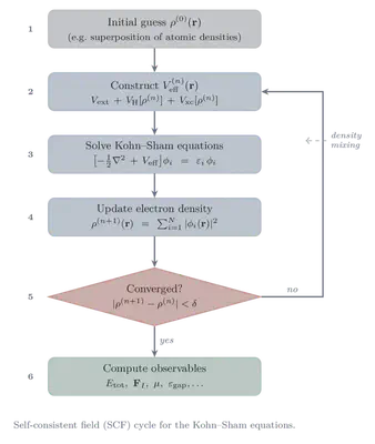
Initialise: Start with an initial guess for the electron density $\rho^{(0)}(\mathbf{r})$ (commonly taken from a superposition of atomic densities).
Build the potential: Construct $V_{\mathrm{eff}}^{(n)}(\mathbf{r})$ from the current density $\rho^{(n)}$ using equation \eqref{eq:Veff}.
Solve the KS equations: Diagonalise the KS Hamiltonian
$\hat{H}_{KS}= -\frac{1}{2}\nabla^2 + V_{\mathrm{eff}}^{(n)}$
to obtain the updated orbitals $\phi_i^{(n)}(\mathbf{r})$ and eigenvalues $\epsilon_i^{(n)}$.
Update the density: Form the new density: \begin{equation} \rho^{(n+1)}(\mathbf{r}) = \sum_{i=1}^N |\phi_i^{(n)}(\mathbf{r})|^2. \end{equation}
Check convergence: If $\rho^{(n+1)} \approx \rho^{(n)}$ (to within a chosen threshold, e.g. in total energy or charge density norm), the SCF loop has converged. Otherwise, set $n \gets n+1$ and return to step 2.
In practice, direct substitution $\rho^{(n+1)} \to \rho^{(n)}$ often converges slowly or not at all. Sophisticated density mixing schemes (Pulay/DIIS mixing, Broyden mixing) are used to accelerate convergence by extrapolating from several previous iterations.
Approximations to $E_{\mathrm{xc}}$
The KS formalism is formally exact — all approximations enter solely through the choice of $E_{\mathrm{xc}}[\rho]$. The quality of a DFT calculation therefore rests on the quality of the XC approximation. Common choices, in increasing order of sophistication (the “Jacob’s Ladder” of DFT), include:
Local Density Approximation (LDA): $E_{\mathrm{xc}}^{\mathrm{LDA}}[\rho] = \int \varepsilon_{\mathrm{xc}}(\rho(\mathbf{r})),\rho(\mathbf{r}),d\mathbf{r}$, where $\varepsilon_{\mathrm{xc}}$ is the XC energy per electron of a uniform electron gas at density $\rho$. Accurate for slowly varying densities; systematically overbinds.
Generalised Gradient Approximation (GGA): Adds dependence on the gradient $\nabla\rho(\mathbf{r})$ to account for density inhomogeneity (e.g. PBE functional). Significantly improves over LDA for molecules and surfaces.
Hybrid functionals: Mix a fraction of exact Hartree–Fock exchange with GGA correlation (e.g. B3LYP, HSE06). More accurate for band gaps and molecular properties, but computationally more expensive.
Meta-GGA, RPA, double hybrids: Higher rungs of the Jacob’s Ladder incorporate kinetic energy density, non-local correlation, or perturbation theory corrections.
The choice of functional is system-dependent and is one of the primary sources of error in practical DFT calculations.
Physical Interpretation of the KS Eigenvalues
A common point of confusion is the meaning of the Lagrange multipliers $\epsilon_i$ — the KS eigenvalues. They are not the true quasiparticle excitation energies of the interacting system; they arise as mathematical parameters enforcing orbital orthonormality.
However, there are two rigorous statements:
Koopmans-like theorem (exact DFT): The eigenvalue of the highest occupied KS orbital (HOMO), $\epsilon_N$, equals the negative of the exact ionisation energy of the system: $\epsilon_N = -I$. This is an exact result in DFT (unlike in Hartree–Fock where it is only approximate).
All other eigenvalues $\epsilon_i$ ($i < N$) have no rigorous physical interpretation in terms of excitation energies. In practice they are widely (and somewhat informally) used to interpret band structures, density of states, and orbital energies, and often agree qualitatively with experiment, but this agreement is not guaranteed by the theory.
Formally correct excitation spectra require going beyond ground-state DFT, e.g. via Time-Dependent DFT (TDDFT) or many-body perturbation theory (GW approximation).
Summary
The Kohn–Sham scheme reduces the interacting many-body problem to a set of effective single-particle equations \eqref{eq:KS-eqn} that can be solved efficiently on modern computers. The key steps and ideas are:
| Concept | Role |
|---|---|
| Non-interacting reference system | Enables exact computation of $T_s[\rho]$ via orbitals |
| $V_{\mathrm{H}}$ | Classical mean-field Coulomb repulsion, computed exactly |
| $V_{\mathrm{xc}}$ | All many-body quantum effects, must be approximated |
| SCF loop | Resolves the self-consistency between density and potential |
| XC approximation (LDA, GGA, …) | The only uncontrolled approximation in the KS framework |
The formal exactness of the KS framework — all errors traceable to a single approximated term — combined with its single-particle structure makes DFT the workhorse of electronic structure theory. In the chapters that follow, we will examine how this framework is implemented in practice: basis sets, pseudopotentials, $k$-point sampling, and the computational details of solving the KS equations for real materials.