Introduction

The density functional theory (DFT) has established itself as the primary tool to calculate the electronic structure of materials.

The method is at its heart is a method to minimize the Helmholtz Free energy using variational principle. The Helmholtz energy of a system is a functional of the density and minimizing Helmholtz energy gives us the equilibrium density.

The DFT for electronic structure calculation takes the eigen value of the Schrödinger’s equation as a functional of charge density.

Schrödinger’s Equation: revisit for multi-particles system

The Schrödinger equation is the driver equation for quantum mechanical system \begin{equation} \left[\frac{\hbar^2}{2m}\nabla^2+V(r)\right]\Psi(r)=E\Psi(r) \end{equation}

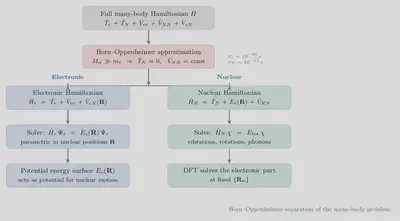
The problem arises when there is many particles in the system. In this case, The manybody Hamiltonian for N nucleus and n electrons is:

Now, the time independent Hamiltonian $\hat{H}=H(p,q)$ is function of two vectors $p,q$ the solution of the problem becomes increasingly difficult when we deal with more than one-electron systems.

Even for a simple system like O, with 8 electrons, and we take very rough data of 10 points in each coordinates, we need $10^{24}$ data points. In modern computers, for each each real numbers we need 64 bit memory. Hence, to store the data of one O atom, we need $64\times 10^{24}$ bit $8\times 10^{24} \mathsf{bit}\approx 10^{17}$MB. (To understand how big this number is, try to find out the age of universe in second!!!)

So we need some approximations to solve the problem.

Born-Oppenheimer Approximation

Given the fact that the protons are $\approx 10^3$ times heavier than electrons, under the same field, it moves much slower than electrons. That raises the Born-Oppenheimer (BO) approximations, where we freeze the motion of nucleus.

In the equation above, that means, $\frac{\hbar}{2M_j}\sum_j^N\nabla^2_j = 0$, $\frac{1}{2}\sum\frac{Z_iZ_j}{|{R_i-R_j}|}=constant$ and $\sum\frac{Z_i}{|\mathbf{r}_i-\mathbf{R}_j|}$ is a function of $r$ only.

So, the Hamiltonian is \begin{align*} \hat{H} =&-\frac{\hbar^2}{2m}\sum_{i}^n\nabla^2_i & \mbox{Kinetic Energy of e}\newline &+ \frac{1}{2}\sum_{i\neq j}\frac{1}{|\mathbf{r}_i-\mathbf{r}_j|} &\mbox{PE of e}\newline & +v_0(r) & \mbox{PE of e due to nucleus} \end{align*}

Mean Field Approximation

Hartree Approximation

After the BO, we are still leaving with the fact that the main problematic variable, i.e. PE(e) is still there. We now approximate the variable.

The obvious first approximation is that of non-interacting electrons, which means the electrons doesn’t interact with each other, which gives PE(e)=0. But this gives a gross incorrect result.

To solve this, we approximate that all $e$s are in a “mean” field created by all the electrons. Legitimately, this approximation is called the mean field, or by the name of the proposer, Hartree approximation.

By this, we can replace the PE(e) as \begin{equation} \frac{1}{2}\sum_{i\neq j}\frac{1}{|\mathbf{r}_i-\mathbf{r}_j|} = \int dr \frac{\rho(r,r’)}{|r_i-r’|}=U_H \end{equation}

So, we have the final Hamiltonian:

\begin{align*} \hat{H}=-\frac{\hbar^2}{2m}\sum_{i}^n\nabla^2_i + \int dr \frac{\rho(r,r’)}{|r_i-r’|} +v_0(r) \end{align*}

Hartree-Fock Approximation

Hartree approximation is not perfect, as it did not take into account that $e$ has spin and obeys Pauli’s exclusion. Fock incorporated that, resulting the Hartree-Fock approximation.

HF method anti-symmetrizes the $\Psi$

$$ \Psi(r_1,r_2\cdots r_N)= \frac{1}{\sqrt{N}}\begin{bmatrix} \psi_1(r_1) &\cdots &\psi_1(r_N)\\ \vdots & \ddots & \vdots\\ \psi_N(r_1) &\cdots &\psi_N(r_N)\\ \end{bmatrix} $$ and solve it using variational method: